Right Riemann Sums: Master It With This Easy Guide!

Delving into the world of integral calculus can feel daunting, but fear not! Understanding Riemann Sums, a cornerstone of approximation techniques, is surprisingly accessible. MathIsFun.com provides excellent interactive resources for visualizing these concepts. This guide helps you tackle how to do a right riemann sum effectively. This method helps solve complex integration problems where the Fundamental Theorem of Calculus can't do the job. From partitioning intervals to calculating areas, learn how to do a right riemann sum with confidence. Khan Academy offers free tutorials on related topics to strengthen your understanding of the underlying math principles.

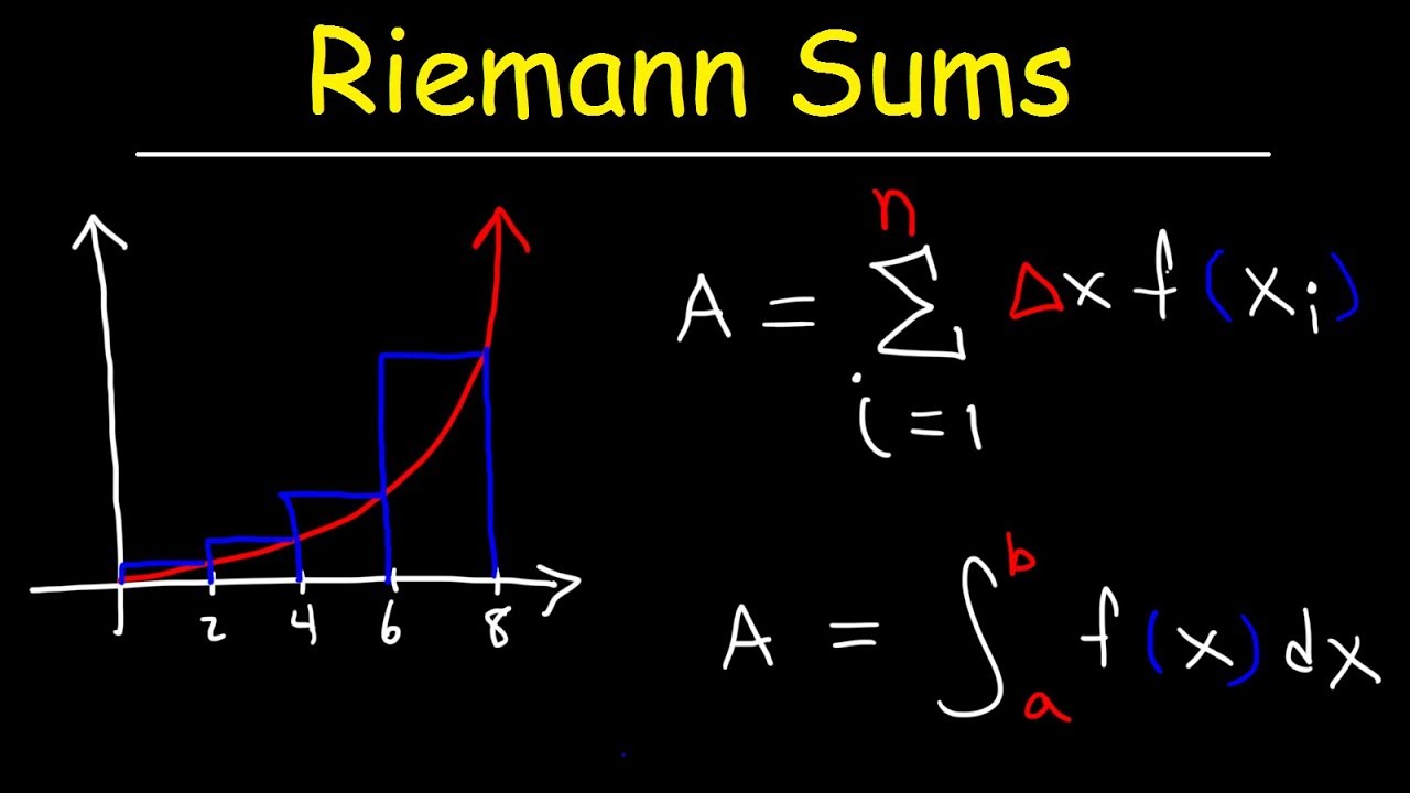
Image taken from the YouTube channel The Organic Chemistry Tutor , from the video titled Riemann Sums - Left Endpoints and Right Endpoints .

Unveiling the Power of Riemann Sums

Imagine trying to find the area of a shape, not a perfect square or circle, but something irregular and curved. This is where the beauty and power of Riemann Sums come into play.

Riemann Sums provide a fundamental tool for approximating the area under a curve, a concept that has far-reaching implications in various fields, from physics and engineering to economics and statistics. They are essential for understanding the foundations of integral calculus.

The Significance of Area Under a Curve

The area under a curve isn't just a geometric concept; it represents accumulated quantities. For instance, if the curve represents the velocity of an object over time, the area under the curve represents the total distance traveled.

Similarly, in economics, it could represent consumer surplus, and in probability, it relates to probabilities within a continuous distribution. This makes calculating the area under a curve incredibly valuable.

Riemann Sums: Approximating the Complex

So, what exactly are Riemann Sums? They are a method of approximating the area under a curve by dividing the area into a series of rectangles.

Each rectangle's area is easily calculated (width × height), and the sum of these rectangular areas provides an estimate of the total area under the curve.

The more rectangles we use, the better the approximation becomes. Think of it as zooming in on a digital image – the more pixels, the clearer the picture. This process allows us to tackle complex shapes, breaking them down into manageable, simpler forms.

Demystifying the Right Riemann Sum

While there are different types of Riemann Sums, we'll focus on the Right Riemann Sum. In this method, the height of each rectangle is determined by the value of the function at the right endpoint of each subinterval.

Don't worry if that sounds confusing right now. We'll break down each of these terms, providing a step-by-step approach to understanding and calculating Right Riemann Sums. By the end, you'll have a solid grasp of this crucial concept.

Unlocking the secrets of Riemann Sums requires a solid foundation. Much like constructing a building, you need to lay the groundwork before you can start building upwards. Let's delve into these essential concepts that form the bedrock of understanding Right Riemann Sums, ensuring you're well-equipped for the journey ahead.

Understanding the Fundamentals: Building Blocks for Success

At its core, understanding Right Riemann Sums involves grasping a few fundamental concepts. These concepts are the essential building blocks. We'll explore intervals, functions, partitions, and how to calculate the width of subintervals.

Defining the Interval and the Function (f(x))

The interval defines the boundaries over which we're calculating the area under the curve.

Think of it as the section of the x-axis we're interested in. It is typically denoted as [a, b], where a is the starting point and b is the ending point.

The function, f(x), describes the curve itself. It tells us the height of the curve at any given point x within our interval.

Without a clearly defined interval and function, calculating the area under the curve would be impossible. They are the starting point of our journey.

Explaining Partition and How to Divide the Interval

A partition is simply a way of dividing our interval [a, b] into smaller subintervals.

We do this by selecting points within the interval. These points divide the total width into smaller sections.

These sections don't have to be equal.

However, for simplicity, we often aim for subintervals of equal width. This greatly simplifies calculations and makes it easier to apply the Right Riemann Sum method.

Calculating the Width of Subinterval (Δx): A Crucial Step

The width of the subinterval (Δx) is perhaps the most crucial calculation in the Riemann Sum process.

It determines the width of each rectangle we'll use to approximate the area under the curve.

A consistent and accurate Δx is crucial for an accurate calculation.

Here's the formula for calculating Δx when the interval is divided into n equal subintervals:

Δx = (b - a) / n

Where:

• a is the starting point of the interval.
• b is the ending point of the interval.
• n is the number of subintervals.

Example:

Let's say our interval is [0, 4] and we want to divide it into 4 subintervals (n = 4).

Δx = (4 - 0) / 4 = 1.

This means each rectangle will have a width of 1.

Identifying the Endpoint: Why We Choose the Right Endpoint

In a Right Riemann Sum, we specifically use the right endpoint of each subinterval to determine the height of the rectangle.

The function f(x) is evaluated at the right endpoint. This result is then used as the rectangle's height.

Why the right endpoint?

It's a convention, a specific way of approximating the area. Other methods exist. Using the left endpoint, or the midpoint, will give alternative approximations. Each may have different behavior with specific functions.

The key is consistency: stick to the right endpoint throughout the entire calculation when using the Right Riemann Sum.

Mastering these fundamental concepts is the first step towards confidently tackling Right Riemann Sums. With a clear understanding of intervals, functions, partitions, and subinterval widths, you're well on your way to unlocking the power of approximation!

After understanding the foundational elements, we're ready to move towards the core of our exploration: the Right Riemann Sum itself. Imagine transforming the area under a curve into a series of neatly arranged rectangles. By carefully calculating the area of each rectangle and summing them up, we arrive at an approximation of the total area.

The Right Riemann Sum in Action: Step-by-Step Calculation

Let's dive into how to actually calculate a Right Riemann Sum. This involves a series of straightforward steps that, once mastered, will allow you to estimate the area under any curve, within a specified interval.

Finding the Rectangle Heights: Evaluating f(x) at the Right Endpoint

The height of each rectangle is determined by the value of the function, f(x), at the right endpoint of each subinterval.

This is the defining characteristic of the Right Riemann Sum: we always look to the right edge of each slice to determine how tall our rectangle should be.

To find the height, simply plug the x-value of the right endpoint into your function.

For example, if your function is f(x) = x² and the right endpoint of a subinterval is x = 2, then the height of that rectangle would be f(2) = 2² = 4.

Calculating Individual Rectangle Areas

Once you have the height of each rectangle, calculating its area is simple.

Recall that the area of a rectangle is given by:

Area = height × width.

We already know the height (from the previous step) and the width is simply Δx, which we calculated earlier by dividing the interval by n subintervals.

Therefore, the area of each rectangle is:

Area = f(right endpoint) × Δx

Summation Notation: Expressing the Riemann Sum Formally

As you might imagine, if we have many rectangles, writing out the sum of their areas can become quite tedious.

This is where summation notation, also known as Sigma notation, comes to our rescue.

Sigma notation provides a compact and elegant way to represent the sum of a series of terms.

The Greek letter Sigma (Σ) is used to denote summation. Here's a breakdown of the notation:

• Σ: The summation symbol.
• i = 1: The index of summation, starting at 1.
• n: The upper limit of summation (the total number of subintervals/rectangles).
• f(xi)Δx: The expression being summed (the area of each rectangle).

Therefore, the Riemann Sum can be written as:

∑(i=1)^n▒f(xi )Δx

This expression tells us to add up the areas of all the rectangles, starting from the first rectangle (i = 1) and continuing until the nth rectangle.

The Right Riemann Sum Formula

Putting it all together, here's the formula for the Right Riemann Sum:

Right Riemann Sum = Σ(i=1)^n▒f(xi )Δx = Δx [f(x1) + f(x2) + ... + f(x

_n)]

Where:

• n is the number of subintervals.
• Δx is the width of each subinterval.
• x_i is the right endpoint of the ith subinterval.
• f(x_i) is the value of the function at the right endpoint of the ith subinterval (the height of the ith rectangle).

This formula provides a concise and powerful way to calculate the Right Riemann Sum, allowing us to approximate the area under a curve with increasing accuracy as we increase the number of subintervals.

After understanding the mechanics of the Right Riemann Sum, it's time to solidify that knowledge through application. Theory is crucial, but seeing the process unfold in a tangible example truly cements the concepts and builds confidence. Let's put our newfound skills to the test.

Example Time: Let's Work Through It Together!

Let's dive into a concrete example to see the Right Riemann Sum in action. We'll choose a simple function and interval to illustrate each step clearly. By working through this example together, you'll gain a deeper understanding of the process and develop the confidence to tackle more complex problems.

Setting Up Our Example

First, we need to define our playing field. Let's consider the function f(x) = x² on the interval [0, 2].

This means we want to approximate the area under the curve of f(x) = x² between x = 0 and x = 2. To keep things simple, let's use n = 4 subintervals. This will give us four rectangles to work with.

Step-by-Step Calculation: Unveiling the Process

Now, let's break down the calculation into manageable steps:

1. Finding Δx (Width of Subinterval):

   Recall that Δx is calculated as (b - a) / n, where 'a' is the starting point of the interval, 'b' is the ending point, and 'n' is the number of subintervals. In our case, a = 0, b = 2, and n = 4. Therefore, Δx = (2 - 0) / 4 = 0.5. Each rectangle will have a width of 0.5.

2. Identifying the Right Endpoints:

   Since we're using the Right Riemann Sum, we need to find the x-values of the right endpoints of each subinterval. Our subintervals are: [0, 0.5], [0.5, 1], [1, 1.5], and [1.5, 2]. The right endpoints are therefore: 0.5, 1, 1.5, and 2.

3. Calculating Rectangle Heights:

   To find the height of each rectangle, we need to evaluate the function f(x) = x² at each right endpoint.

   • f(0.5) = (0.5)² = 0.25
   • f(1) = (1)² = 1
   • f(1.5) = (1.5)² = 2.25
   • f(2) = (2)² = 4

4. Calculating Individual Rectangle Areas:

   Now we can find the area of each rectangle using the formula: Area = height × width.

   • Rectangle 1: Area = 0.25 × 0.5 = 0.125
   • Rectangle 2: Area = 1 × 0.5 = 0.5
   • Rectangle 3: Area = 2.25 × 0.5 = 1.125
   • Rectangle 4: Area = 4 × 0.5 = 2

5. Summing the Areas:

   Finally, we add up the areas of all the rectangles to get our Right Riemann Sum approximation. Right Riemann Sum ≈ 0.125 + 0.5 + 1.125 + 2 = 3.75

   Therefore, our approximation of the area under the curve f(x) = x² from x = 0 to x = 2, using a Right Riemann Sum with 4 subintervals, is 3.75.

Visualizing the Approximation

Imagine a graph of f(x) = x² from x = 0 to x = 2. Now, picture four rectangles sitting under the curve. Each rectangle's width is 0.5, and its height touches the curve at the right edge of each section.

You'll notice that in some places, the rectangles overshoot the curve, and in others, they fall short. This overestimation and underestimation contribute to the approximation we calculated. A visual representation makes it clear why this is an approximation, not an exact area.

Comparing to the Definite Integral

To understand how good our approximation is, let's calculate the definite integral of f(x) = x² from 0 to 2. The definite integral gives us the exact area under the curve.

The definite integral of x² is (x³/3). Evaluating this from 0 to 2 gives us: [(2)³/3] - [(0)³/3] = 8/3 ≈ 2.67.

Notice that our Right Riemann Sum approximation (3.75) is higher than the actual area (2.67). This is because, in this particular example, the function is increasing over the interval, causing the right endpoints to overestimate the area.

The difference between the approximation and the exact value highlights the inherent error in Riemann Sums. By increasing the number of subintervals (making n larger), we can reduce the width of each rectangle and achieve a more accurate approximation.

After understanding the mechanics of the Right Riemann Sum, it's time to solidify that knowledge through application. Theory is crucial, but seeing the process unfold in a tangible example truly cements the concepts and builds confidence. Let's put our newfound skills to the test.

Connecting the Dots: From Riemann Sums to Definite Integrals

Riemann Sums, particularly the Right Riemann Sum, are not just abstract mathematical exercises. They are a vital stepping stone to understanding one of the most powerful concepts in calculus: the Definite Integral. Let's explore this connection and unravel the deeper meaning behind the approximation.

Riemann Sums as Approximations of the Definite Integral

Think of the Right Riemann Sum as a way to estimate the area under a curve by dividing it into rectangles. The more rectangles we use (the larger 'n' becomes), the better our approximation gets.

The Definite Integral, on the other hand, represents the exact area under the curve. It is the value that the Riemann Sum approaches as the number of rectangles approaches infinity. In essence, the Definite Integral is the limit of the Riemann Sum.

The Integral Symbol (∫): A Gateway to Exactness

The integral symbol, ∫, might look like a stretched-out "S," and that's no accident! It stands for "sum." But it's not just any sum; it's the continuous sum that gives us the exact area under the curve.

The Definite Integral is written as:

∫ab f(x) dx

Where:

• 'a' and 'b' are the limits of integration (the interval over which we are finding the area).
• f(x) is the function defining the curve.
• dx represents an infinitesimally small width.

This notation formalizes the idea of summing an infinite number of infinitely thin rectangles.

The Power of the Limit

The key to understanding the relationship lies in the concept of a limit. As the number of subintervals (n) in the Riemann Sum approaches infinity, the width of each subinterval (Δx) approaches zero.

This means that our approximation becomes increasingly accurate, ultimately converging to the true area under the curve. We express this mathematically as:

limn→∞ ∑i=1n f(xi) Δx = ∫ab f(x) dx

This equation states that the limit of the Riemann Sum as n approaches infinity equals the Definite Integral.

Calculus Significance

The connection between Riemann Sums and Definite Integrals is fundamental to integral calculus. It provides a rigorous way to define and calculate areas, volumes, and other quantities.

It bridges the gap between discrete approximations and continuous functions.

Understanding this connection opens doors to a vast array of applications in physics, engineering, economics, and other fields. Mastering Riemann Sums empowers you to tackle complex problems by breaking them down into manageable approximations, paving the way for precise solutions through the magic of calculus.

After seeing how Right Riemann Sums connect to Definite Integrals, it's natural to wonder if there are other ways to approach this approximation. The world of Riemann Sums extends beyond just the right endpoint, offering different perspectives on estimating the area under a curve. Exploring these variations enriches our understanding and provides a more complete picture of the underlying principles.

Beyond the Right: Exploring Other Riemann Sum Variations

While the Right Riemann Sum uses the right endpoint of each subinterval to determine the rectangle's height, it's not the only game in town. There are other legitimate, and sometimes even better, ways to build our rectangles and approximate that area. Let's peek at two common variations: the Left Riemann Sum and the Midpoint Riemann Sum.

Left Riemann Sum: A Different Perspective

The Left Riemann Sum offers a contrasting approach. Instead of using the right endpoint of each subinterval to determine the height of the rectangle, it uses the left endpoint.

Imagine our familiar curve divided into rectangles. With the Left Riemann Sum, the height of each rectangle is determined by the function's value at the left edge of that rectangle.

This simple change in perspective can lead to noticeable differences in the approximation, especially when the function is rapidly increasing or decreasing. The formula for the Left Riemann Sum adjusts to reflect this:

∑ni=1 f(xi−1)Δx

Midpoint Riemann Sum: Seeking Balance

The Midpoint Riemann Sum attempts to strike a balance between the overestimation and underestimation that can occur with the Left and Right Riemann Sums. As the name suggests, it uses the midpoint of each subinterval to determine the rectangle's height.

This method often provides a more accurate approximation than either the Left or Right Riemann Sum, as it tends to average out the errors. It's like aiming for the center of the target instead of consistently hitting to one side. The formula becomes:

∑ni=1 f(xi∗)Δx

Where x_i is the midpoint of the i*th subinterval.

Choosing the Right Approach: When Does It Matter?

So, which Riemann Sum variation should you use? The answer, as with many things in calculus, depends on the specific function and the desired level of accuracy.

• If the function is monotonically increasing (always increasing) over the interval, the Left Riemann Sum will underestimate the area, and the Right Riemann Sum will overestimate it.
• Conversely, if the function is monotonically decreasing (always decreasing), the Left Riemann Sum will overestimate the area, and the Right Riemann Sum will underestimate it.
• The Midpoint Riemann Sum often provides a better approximation in both cases, as it tends to balance out the errors.

In situations where higher accuracy is paramount, or when dealing with functions that change direction frequently, the Midpoint Rule is often preferred. Furthermore, when approximating definite integrals numerically, more sophisticated techniques like Simpson's Rule, which builds on the ideas of Riemann Sums, offer even greater precision. Each method offers a unique lens through which we can view and approximate the area under a curve.

After seeing how Right Riemann Sums connect to Definite Integrals, it's natural to wonder if there are other ways to approach this approximation. The world of Riemann Sums extends beyond just the right endpoint, offering different perspectives on estimating the area under a curve. Exploring these variations enriches our understanding and provides a more complete picture of the underlying principles.

Tips, Tricks, and Common Mistakes to Avoid

Calculating Right Riemann Sums can be a straightforward process, but it's easy to stumble along the way. Let's explore some strategies to refine your approach, prevent errors, and enhance the accuracy of your approximations. With a few key insights, you'll navigate these calculations with greater confidence and precision.

Optimizing Accuracy: Choosing the Right Number of Subintervals

The accuracy of a Riemann Sum hinges on the number of subintervals you use. More subintervals generally lead to a more accurate approximation because the rectangles more closely conform to the curve of the function.

However, there's a trade-off. More subintervals mean more calculations. Aim for a balance – enough subintervals to achieve acceptable accuracy without making the process overly cumbersome.

Think of it like pixels in a digital image: more pixels create a sharper picture.

As you experiment with different numbers of subintervals, observe how the Riemann Sum converges toward a stable value. This can give you a sense of when you've reached a point of diminishing returns, where adding more subintervals provides only marginal improvements in accuracy.

Spotting the Pitfalls: Common Mistakes to Avoid

Even with a solid understanding of the concepts, errors can creep into your calculations. Recognizing and avoiding these common pitfalls is essential for obtaining reliable results.

The Dreaded Δx Calculation Error

The width of the subinterval (Δx) is a foundational element of the Riemann Sum calculation. An incorrect Δx will throw off all subsequent calculations. Double-check your formula (Δx = (b - a) / n) and ensure you're using the correct interval endpoints (a and b) and the number of subintervals (n).

Function Misinterpretation

Ensure you're evaluating the function (f(x)) correctly at the right endpoints. Pay close attention to the function's equation and be mindful of order of operations. For complex functions, it can be helpful to break down the evaluation into smaller, manageable steps.

Endpoint Identification Issues

Specifically for Right Riemann Sums, be certain that you are using the right endpoint of each subinterval to determine the height of the rectangle. A simple mistake here can lead to a Left Riemann Sum calculation instead!

Forgetting Summation

Don't forget to sum the areas of all the rectangles! The Riemann Sum is the sum of the areas of all the individual approximating rectangles, and a single missing rectangle will compromise your final result.

Tools for Success: Leveraging Online Calculators and Software

Fortunately, you don't have to perform these calculations entirely by hand. Numerous tools and resources are available to assist you:

• Online Riemann Sum Calculators: Several websites offer calculators that can compute Riemann Sums for you, given a function, interval, and number of subintervals. These are useful for checking your work and experimenting with different parameters.

• Computer Algebra Systems (CAS): Software like Mathematica, Maple, or even Python with libraries like NumPy and SciPy can perform symbolic and numerical calculations, including Riemann Sums and definite integrals. These tools are particularly helpful for complex functions or when high accuracy is required.

• Graphing Calculators: Many graphing calculators have built-in functions for calculating Riemann Sums. Consult your calculator's manual for instructions.

• Spreadsheet Software: Programs like Microsoft Excel or Google Sheets can be used to organize and perform the calculations involved in Riemann Sums. You can create columns for the endpoints, function values, rectangle areas, and the running sum.

By mastering these tips, tricks, and by being aware of common pitfalls, you'll be well-equipped to tackle Right Riemann Sum calculations with confidence and precision. The resources available further enhance your ability to explore and understand this fundamental concept in calculus.

Video: Right Riemann Sums: Master It With This Easy Guide!

Play Video